BIO EN/CS 6640 Introduction to Image Processing - Extension

Zach Gildersleeve
April 4, 2007

Minimum Squared Error Template Matching Applied to Image Stitching

script used: stitch.m

The following discusses the script stitch.m, which generates a stitched image from two different but related images using minimum squared error template matching in the fourier domain, and affine transformation estimation and deriving in the spatial domain. The discussion, and the associated script is limited to these areas, so many shortcuts are taken, including using grayscale images, using few points of error registration (typically only two), and so on as will be seen. Most of what is discussed can easily be expanded upon, so we will only be interested in stitching two images. Additional images could be stitched by running the script multiple times with different images.

Initially, the two images are read in as a format that MatLab handles (a matrix of doubles) and each image is squared. The two images are displayed, and the user is prompted to select a number of points on the first image (image1). This feature could be used to allow the user to select matching points in the second image (image2), but we will use template matching for this purpose instead and the points themselves are hard coded. Two points are used, which allow for quick registration and affine estimation, but additional points could be used. Each additional point creates a more robust translation matrix.

The user selected points are stored in two arrays, userX and userY which together hold the point set (userX, userY). The matching set of points will be found using minimum squared error template matching in the fourier domain. To estimate the affine transformation from one image to another, we use a subimage of image1, a square set of pixels with the user selected point as the top left corner. The goal is to then find the subimage in image2 by "sliding" the subimage over the. At each location the difference between the subimage and the pixels in image2 is squared, and the minimum difference represents the point of best match. In the spatial domain, this is seen as:

At this point in the derivation, we can see that the term we are interested in is the second term, as the first term is the sum of the square of image2, and the third term is the sum of the square of the shifted subimage. It is also worth noting that this term is very similar to the definition of convolution of two images in the spatial domain, which we know as multiplication in the frequency domain.

To solve this term in the frequency domain, first it is necessary to pad the subimage out to make it the same size as image2. A mask this same size is created which will be used to combine the padded subimage and image2. The fourier transform of image1, image2, the padded subimage, and the mask is found using the fast fourier transform. Using term by term multiplication of the squared image with the complex conjugate of the mask, we acquire a resulting matrix that represents the three terms for each pixel location. The minimum value of this matrix, in image coordinates, are the coordinates of the minimum error, and thus are the coordinates in image2 where the image1 pixel at (userX, userY) best matches given the size of the subimage. This resulting coordinate set, for multiple points, is then stored in (Xoffset1, Yoffset1) and (Xoffset2, Yoffset2), where the first set should match the coordinates in (userX, userY).

Initial Affine Transformation Estimation

Initially, the transformation to transform image1 to image2 via the identified points can be estimated by a building a simple matrix from the points and solving. This solution is not fully correct, and the complete affine derivation will be explored below that should offer a more robust transformation matrix. Initially, through, we assume that the transformation between image1 and image2 is affine, or more accurately, we only solve for this transformation, and ignore lens and focal plane distortion, and perspective transformations. However it is possible, given a small number of points, to estimate this transformation - the transformation to transform (Xoffset1, Yoffset1) to (Xoffset2, Yoffset2) and we assume the rest of the image correctly around these points. To solve for the transformation matrix, we build a matrix out of the sets of points, and left divide to get the resulting matrix values, which are then used to fill out the transformation matrix. The below derivation illustrates how this is accomplished. It is important to remember that Xoffset1, etc. are vectors that contain numberOfPoints values.

This transformation matrix can then be used to transform image2, which is interpolated and rebuilt in transformedImage.

The final step is to draw image1 and transformedImage in the same coordinate system. Exactly how this is done is determined by whether transformedImage is greater than or less than in coordinate space, meaning whether image2 is above and/or to the left (negative) or below and/or to the right (positive).

Initial Results

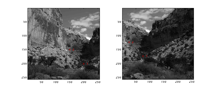
The below images represent the results from the implemented algorithm, using two points for the template matching and the above affine estimation. In all the results, the two matching points are indicated by red crosses. The first set of images are taken from a single image that is split up by a simple translation, therefore there should be zero error between the two images, and the final stitched images should be identical to the original image (excluding floating point and rounding error). As we can see, the stitched image is very nearly seamless.

initial two images

resulting stitched image

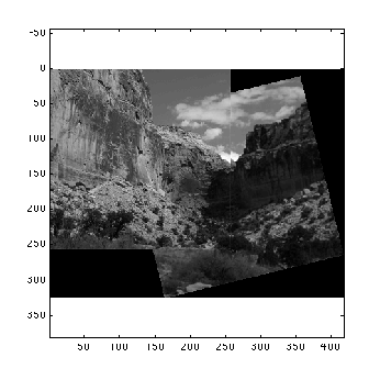
The next set of images is again pulled from the same photograph, but the second image is offset by 2D translation and rotation. The two images are stitched together correctly, but we see that rounding error is more an issue here.

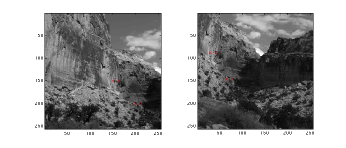notice rotation

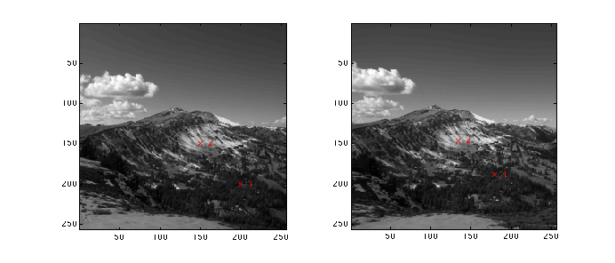
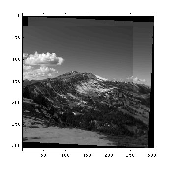
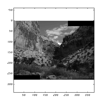
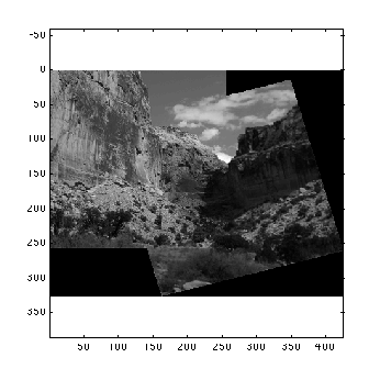
The implemented algorithm was then applied to several sets of images that had unknown distortion. These images are two separate photographs that were taken in the same location, but not controlling for rotation around a common nodal point, as would typically done with a panorama tripod head. In the below image set, the difference between the two images is apparent in the immediate foreground. The stitched image has some of the same errors encountered in the above canyon set with translation and rotation, but the image registration and stitching is relatively successful.

Complete Affine Transformation Derivation

The above images represent the estimated affine transformation. As seen, some misalignments exist from the transformation matrix used to stitch the images. Now we shall explore the complete derivation of the affine transformation, which hopefully will offer a more robust matrix, and remove these alignment errors.

We define p1 and p2 as matrix variables that hold our identified coordinate points. These two matrices are essentially redefinitions of the above P1 and P2. We then reintroduce transformation matrix A. Here we are solving for six values in A (a, b, c, d, x, y) rather than the four above, so we expect a more correct solution. Solving for A is done by finding the minimum A according to the expression below.

Solving for this minimum value for all six elements is a difficult problem. However, we can rewrite the minimum sum as a trace, as below, which is solvable for A using the derivative of the trace.

Expanding and rewriting the trace, and taking the derivative with respect to A, we solve for A by setting the derivative of the trace equal to zero.

This gives us the transformation matrix A, in the form desired above. This matrix, or A' depending on its use, can be used in the implemented stitching algorithm, replacing the previously calculated value of A.

Final Results

Below are the same set of images as used above. We will ignore the registration images, as they are the same, and focus only on the stitched image. The resulting image from the initial affine transformation estimation will be reproduced here, for side by side comparison.

Initial Estimated Results	Derived Results

For a straight translation, both methods produce similar results, with only a slight variation in rotation between the two stitched images. This difference could be the result of round off error and floating point precision. Compared with the original image, though, the derived result is more correct. The difference between the two transformations is more accessible with the translated and rotated image.

Initial Estimated Results	Derived Results

Here the derived results reduces the error experienced in the initial image almost completely.

Conclusions

Although additional work is needed, it is possible to see the differences between the original estimated transformation matrix and the complete derived matrix. The implemented algorithm is not robust for all stitchable images, and more complex distortions such as camera lens distortion, focus issues, and not rotating around the focal node point across sets of pictures can produce incorrect results. Additionally, although every possible point in image1 that corresponds to a template matched point in image2 should produce the same transformation matrix during run time, there are unaccountable differences across sets of points. However, the results immediately above, when compared to the initial estimated results, illustrate the working algorithm, and a step in the right direction for the derived transformation.