CS 6630 Scientific Visualization - Project 5
Zach Gildersleeve
December 8, 2006
CADE login: gildersl
Graduate level credit
Vector Visualization - Test Volumes
Scripts Used: "vectorVis.tcl"
Files Produced: images
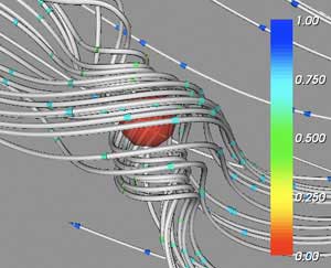
To visualize the vector volume data, several design and implementation choices were made. Each volume dataset has one or more critical points - points where the vector magnitude is very large or very small. Understanding the behavior of these points is the key to understanding the vector volume on a larger scale, and consequentially a detailed analysis of a vector volume might start with these points. To visualize the behavior around the critical points, each point is used as the center of a sphere that provides spawning points for tube streamlines. Using a sphere to generate points allows for a representative sample of the general vector flow, while still generating enough streamlines at a variety of three-dimensional locations to visualize the vector structure as a whole. Cone glyphs are added to the streamlines, and the cones are scaled and colored according to the vector magnitude. While it was never felt that in the current implementation the scaling and coloring corresponds to useable information, a rough idea of the vector magnitude at each glyph location is provided. The cone glyphs are randomly spread around the streamlines, to prevent introducing patterns in the vector volume that do not exist.
It is possible to locate the points where the vector magnitude is very large or very small, and thus the location of critical points, by rendering the magnitude data as a contoured isosurface. This process is detailed in previous assignments, and will not be discussed here. The provided GUI allows for the dynamic shifting of the isosurface contour value, and consequentially each critical point can be quickly identified. This process is further assisted by the manual positioning of a single critical point, which allows the user to match the potential critical point identified as an isosurface, and to view that position as the center of a sphere generating streamlines. A translucent red sphere signifies the location of known critical points. Finally, a red green blue axis locator is drawn centered on the origin (or at the 0, 0, 0 coordinates of the volume) to aid in positioning and orientation.
The following images represent the three test volume datasets, with a description of the known critical point found in each volume.
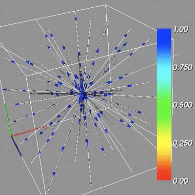
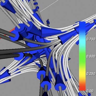
TestVec0, with Repelling Node critical point at (15, 15, 15)
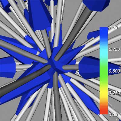
Detail of Repelling Node
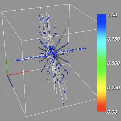
TestVec1, with Saddle Point critical point at (15, 15, 15)
Detail of Saddle Point
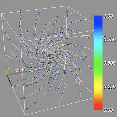
TestVec0, with Attracting Focus critical point at (15, 15, 15)
Detail of Attracting Focus
These three idealized critical point types will serve as a guide for understanding the challenge volume datasets. The workflow for generating the above image for one critical point, including streamlines and cone glyphs, is an extensive process that is outlined below:
structured points dataset -> vtkStructuredPointsReader -> vtkContourFilter -> vtkPolyDataMapper -> isosurface actor
structured points dataset -> vtkStructuredPointsReader + vtkSphereSource + vtkRungeKutta4 -> vtkStreamLine -> vtkRuledSurfaceFilter -> vtkTubeFilter -> vtkPolyDataMapper -> streamline actor
vtkStreamLine + vtkStructuredPointsReader -> vtkProbeFilter -> vtkMaskPoints -> vtkConeSource + vtkGlyph3D -> vtkPolyDataMapper -> cone glyph actor
vtkOutlineFilter -> vtkPolyDataMapper -> bounding box actor
isosurface actor + streamline actor + cone glyph actor + bounding box actor -> vtkRenderer
Vector Visualization - Challenge Volumes
Scripts Used: "vectorVis.tcl"
Files Produced: images
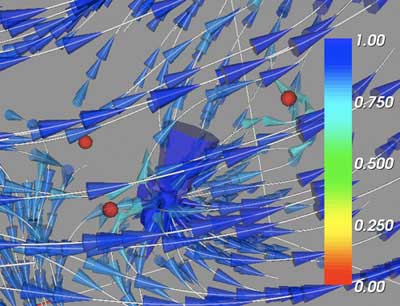
It is possible to extend the above workflow to multiple critical points within a single vector volume. In the two challenge vector volumes, several unknown critical points must be first located by manipulating the isosurface contour value to identify points of interest both at low and high vector magnitudes. Using the sliders, a single critical point can be located. This procedure is repeated for all critical points that are believed to exist. Rendering all identified streamline sources and cone glyphs in the challenge volumes produces the below images. The critical point markers (red translucent spheres) were turned on to aid in identification of each critical point.
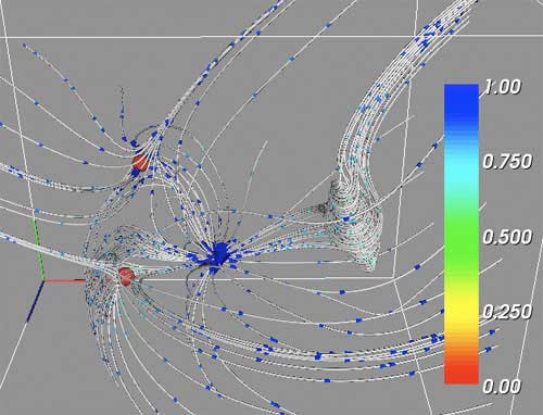 ChalVec0 with four identified critical points |
 ChalVec1 with six identified critical points |
The identified critical points are summarized in the following table.
Dataset |
Number of Critical Points |
Location (X, Y, Z) |
Magnitude |
Type |
ChalVec0 |
4 |
(16.1, 16.8, 25.0) (17.0, 24.5, 13.9) (25.0, 15.0, 18.8) (38.8, 26.1, 32.1) |
Low High High Low |
Saddle Saddle Repelling Attracting |
ChalVec1 |
6 (5) |
( 9.0, 32.0, 16.0) (20.0, 30.0, 20.0) (35.0, 15.0, 20.0) (45.0, 45.0, 20.0) (54.9, 15.2, 20.0) (65.0, 45.0, 20.0) |
? High Low Low Low Low |
Saddle Repelling Attracting Attracting Attracting Attracting |
Each critical point magnitude is ranked according to the isosurface contour value necessary to locate the critical point. The first point listed for ChalVec1 may not be a critical point, as the rest of the dataset has a very defined pattern - that of a high magnitude repelling point shedding low magnitude attracting vortices. The point does have some of the features of a saddle point, but may be more of a construct of the vector volume dataset itself and the implemented means of visualization. It is left in for means of comparison, although an expanded visualization may be necessary to explore this point fully.
Below are some detailed images from the two challenge datasets, showing selected critical points. Again, the located critical point itself is represented as the center of the red sphere.
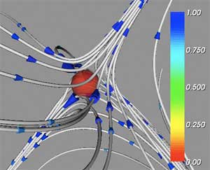 ChalVec0 Saddle at (16.1, 16.8, 25.0) |
 ChalVec0 Attracting at (38.8, 26.1, 32.1) |
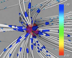 ChalVec1 Repelling at (20.0, 30.0, 20.0) |
 ChalVec1 Attracting at (35.0, 15.0, 20.0 |
Both the saddle and repelling critical point from the challenge datasets match the idealized critical points found in the test volumes, especially at a local level. The attracting focus points do not converge on a single point, but rather around a broader axis when compared to the test volume.
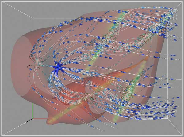
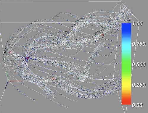
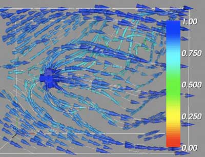
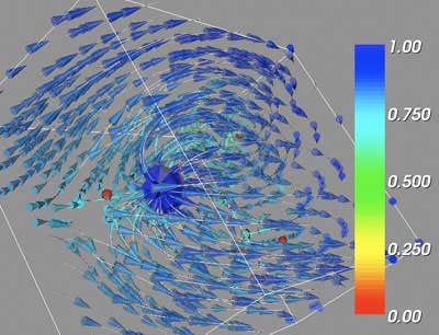
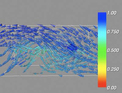
Finally, it is possible to visualize the vector volume as a whole, rather than using the critical points as spawning locations for the streamlines. Instead, we use the bounding box itself to generate streamlines at even locations. The cone glyphs are drawn larger as well, as they provide more three-dimensional location information than the streamlines.
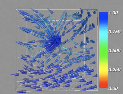
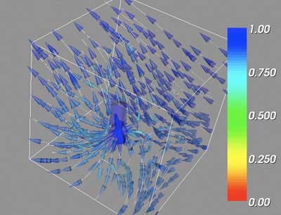
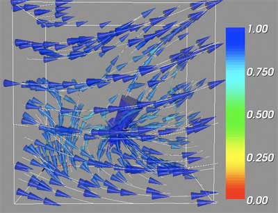
In the above large scale visualizations for ChalVec0, it is possible to see the dominance of the repelling node critical point. With a brief examination, the attracting focus is also evident, but the two saddle points are not reflected in the volume as a whole when rendered under these settings. This is to be expected, as viewing the test volumes using the global streamlines depicts obvious critical points in TestVec0 and TestVec2, the repelling point and attracting focus, but the TestVec1 saddle point is defined by essentially the inverse of the image offered by using the critical point as the streamline source. The story is much the same with ChalVec1. The repelling node dominates the scene, but the attracting focus points are easy to locate with a little effort. Unfortunately, the questionable saddle point is not easily found and does not help to resolve the ambiguities over whether this point is a true critical point, or simply the general location where the vectors "emitting" from the repelling node are swept back with the overall flow of the volume. Nevertheless, the vortex shedding downstream from the repelling node is quite interesting, and promises insight to the vector volume dataset as a whole.
The GUI provides additional control over the vector volume visualizations. The user can select from the three test volumes or the two challenge volumes. Checkboxes allow the user to manually adjust a single critical point location, and use that location as the center of a sphere to generate streamlines. Using this option, additional sliders are revealed that allow to position the streamline generating sphere. Other checkboxes draw the critical point markers as red spheres, or to set the bounding box itself as the source for streamlines rather than the critical points. The number of streamlines can be varied according to the slider, while the number displayed is in groups of the smallest number of points a single sphere can generate. The user can opt to display the streamlines, the isosurface, or both, and can control the isosurface contour value via a slider.
Curl, Curl Magnitude, and Divergence
Scripts Used: "calc.tcl", "vectorCalc.tcl", "vectorCalcVis.tcl"
Files Produced: ChalCMa0.vtk, ChalCMa1.vtk, ChalCur0.vtk, ChalCur0.vtk, ChalDMag0.vtk, ChalDMag0.vtk, images
The following discussion will operate under the below definitions of curl, curl magnitude, and divergence.
Curl is a measurement of the rotation in a vector field around any given axis or any given vector, that is, the angle rotation between two vectors is to be expected.
Curl magnitude is the magnitude of the rotation in the vector field at any given point, or how quickly a vector may rotate around another.
Divergence is a measurement of the quantity and direction of change within a vector field, specifically in terms of whether and how quickly a vector field converges or diverges from a particular point.
The script vectorCalc.tcl operates on challenge volumes 1 and 2, by passing in a command line argument of 0 (vtk vectorCalc.tcl 0) or 1 (vtk vectorCalc.tcl 1) respectively. The script displays the large scale vector visualization presented above, using the bounding box to generate evenly spaced streamlines. These streamlines are placed to provide a sense of location for the isosurface actors, the main focus of this section. Using the slider it is possible to select the contour value to draw an isosurface from the magnitude volume dataset. The magnitude volume is then colormapped through either a volume representing the curl magnitude for each vector location, or the divergence. The script maps the colormap scale bar through the data boundaries.
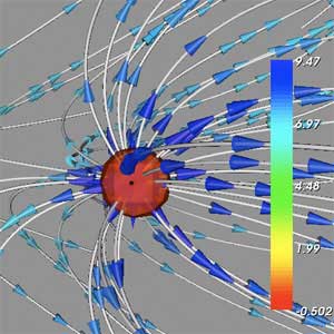
Examining divergence, areas that are associated with repelling critical points generally have a high divergence, which makes sense as high divergence and a repelling node are basically two ways of describing the same feature. There is less a solid association between other critical points and divergence based on the critical point type. For example, the attracting focus critical points are more reliant on their magnitude to predict divergence rather than simply based on their type. In fact, in challenge volume 1, it is possible to make a general observation that there is a direct relationship between the magnitude volume and the divergence volume. When the magnitude is small, a positive divergence (convergent) is a valid assumption; conversely where magnitude is large, a negative divergence (divergent) value is expected. However, this claim does not hold in challenge volume 0, in which negative divergence values are associated with roughly medium magnitude levels. In the images below, the colormapped scale indicates the color that can be attributed to a positive or negative divergence. Despite the high upper boundary for the divergence in each volume, no magnitude value was located that would return these divergence values, and the resulting colors are skewed to the lower end.
 ChalMag0 showing point of low magnitude, with divergence approaching negative values |
 ChalMag0 showing point of high magnitude, with divergence approaching positive values |
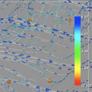 ChalMag1 showing points of low magnitude, with divergence approaching positive values |
 ChalMag1 showing point of high magnitude, with divergence strongly negative |
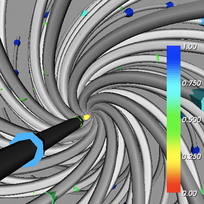
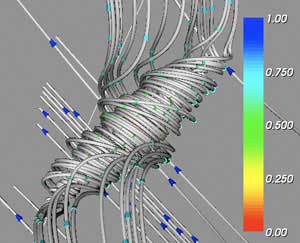
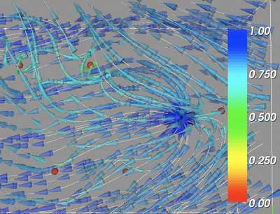
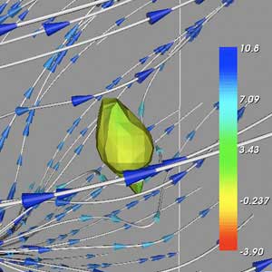
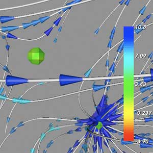
Examining curl, new structures in the field are located. The areas of high curl are generally associated with attractive focus critical points as synonymous with vortices. While the critical points themselves are single point locations, the curl colormap indicates a line that spreads through the axis of the vortex twist (as seen in the far top streamline details). It is difficult to not associate these points of high curl magnitude with the attracting focus vortex locations, but the inclusion of this isosurface with the streamlines adds much to the visualization. These locations are the most significant areas for curl, as the curl magnitude throughout the majority of the volume is fairly similar. The below images show these curl axis locations across the volumes, with the most visible locations of high curl associated with the attracting focus vortices in challenge volume 1.
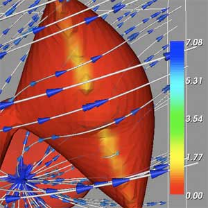 ChalMag0 showing high curve magnitude, associated with a attracting focus vortex |
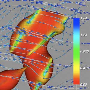 ChalMag1 showing high curve magnitudes, associated with attracting focus vortices |
Finally, including these isosurfaces with the streamlines generated from the critical points adds to the visualization. In vectorCalcVis.tcl (called with command line arguments like vectorCalc.tcl), the user is presented with a combination of the critical point streamlines and the colormapped isosurface. This functionality is included with this script, as it is possible to draw the isosurfaces with the global large scale streamlines with the script vectorCalc.tcl. Divergence information is not readily available from the vector volume, and its inclusion is a benefit. The curl magnitude volume in particular add greatly to the understanding of the underlying volume dataset.