CS 6630 Scientific Visualization - Project 4

Zach Gildersleeve
Nov. 22, 2006

CADE login: gildersl
Graduate level credit

Part 1 - Contour Isosurfaces and Transfer Functions

Scripts Used: "contour.tcl", "volume.tcl"
Files Produced: images

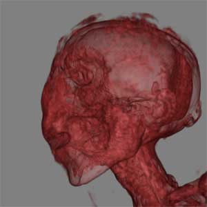
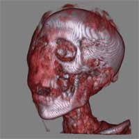
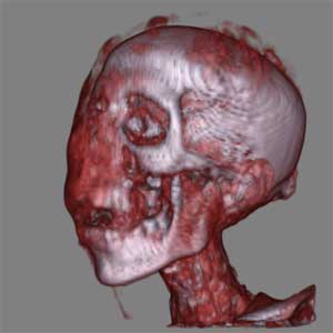
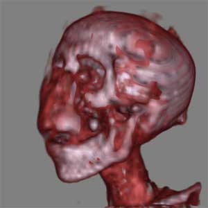
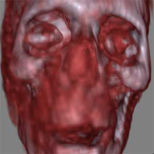
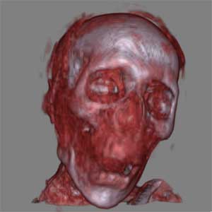Volume rendering of skin and bone	Isosurface values 80 (skin) and 120 (bone)
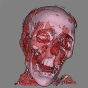
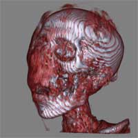
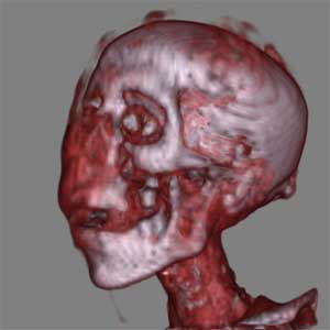
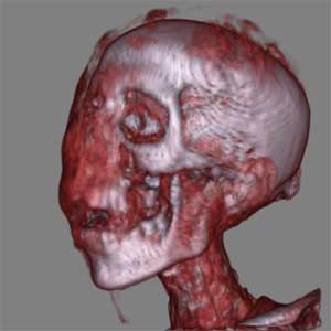
Volume rendering of skin and bone	Isosurface values 80 (skin) and 120 (bone)
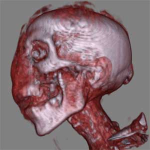
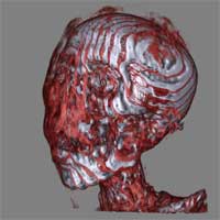
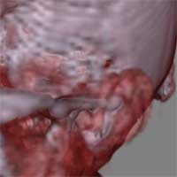
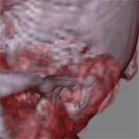
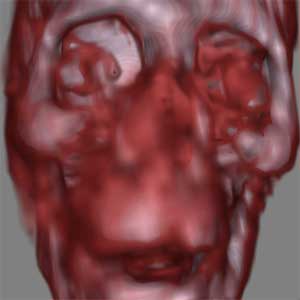
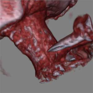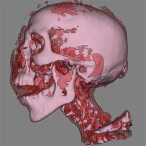
Volume rendering detail	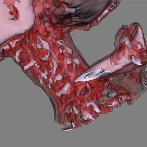Isosurface detail

The script "volume.tcl" creates a transfer function designed to visualize the skin and bone in the mummy dataset. The specific values for the transfer function are established with the use of "contour.tcl," a script used in project 3 to render isosurfaces. An aspect of this script's GUI allows the user to manually set the contour value of the isosurface via a slider. Using this script, it is possible to gain a close approximation as to where the skin and bone density ranges are. Using the isosurface values established for the Visible Man dataset in project 3 do not translate to the mummy dataset, with the mummy overall exhibiting more dense values. After some experimentation, the skin was found to have a density value of between 65 and 105, and the bone between 105 and 210. Other density ranges of note in this dataset are the wrappings, less dense than skin in the range 5 to 60, and the teeth and other very dense bone, like the jaw, that ranges from 220 to the upper limits of the dataset around 250. For the transfer function used in the images above, only the skin and bone were of interest.

The built transfer function (graph and description below) was incorporated into the volume rendering pipeline using the following workflow, with vtkVolume taking the place of the vtkActor used in previous assignments.

vtkPiecewiseFunction & vtkColorTransferFunction -> vtkVolumeProperty + material properties -> vtkVolumeRayCastCompositeFunction

structured points dataset -> structured points reader -> vtkVolumeRayCastMapper + composite function -> vtkVolume -> renderer

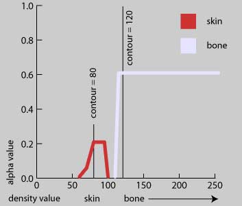
The above graph illustrates the transfer function created for the mummy volume rendering, and indicates where the relative contour values used for the isosurface rendering fall. The skin function assigns values between 60 and 100 an alpha value of 0.2, and a redish color, while the bone function gives all density values greater than 110 a white color and an alpha of 0.6. The 0.2 alpha value for the skin, with the more narrowly defined function, is small enough to composite to a non-opaque value, while the higher alpha value and broader range of the bone function ensures that the bone is visualized as solid and opaque. As any given isosurface maps to a single density value, the two indicated value of 80 and 120 are used in "contour.tcl" to render the isosurface images above. This single value is less a problem with the bone than with the skin. With the bone, the more dense and thus opaque nature goes to an alpha value of 1.0 quickly during volume composting. Visually, this tends to match a single valued isosurface. However, the skin's density range, while not broader than that of bone, has more fluctuation of the number of voxels per any given density. This, with a lower alpha value, leads to visual dissimilarities between the volume rendered skin and the single valued isosurface at 80. This is evident in the detailed images, above, where the volume render emphasizes the existing neck musculature and interior structure.

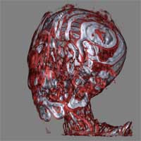
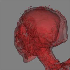Isosurface render of skin only

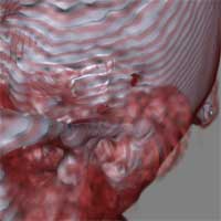
Volume render of skin only

For the mummy dataset, volume rendering offers several advantages over a multiple contour value isosurface visualization. As mentioned above, the most important advantage is the degree to which the softer tissue (skin) is represented. We would expect something like soft tissue to be less binary than bone, and consequentially to produce a softer image that reveals more about the overall structure and state of preservation. The incredible ability of volume rendering to do this over a single isosurface value is clearly evident in the two above images. Both images are only the respective skin function or contour value, rendered without the bone. The volume rendered image shows a variety of detail around the eye, ear, and mouth region that the isosurface simply hides or lacks. The same concept, to a lesser extend, can be applied to the bone only. Naturally, isosurface renderings highlight one specific value, which for certain visualizations would be immensely useful. For the mummy dataset, however, it would be reasonable to expect a more general image that shows the extent of preservation in different anatomical areas to be more relevant and advantageous.

Maximum Intensity Projection Renderings

Script Used: "mip.tcl"
Files Produced: images

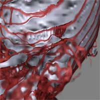
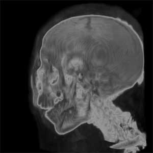MIP ray cast volume render

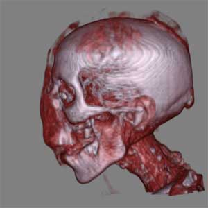Composite based volume render

Using the same pipeline described above, but substituting vtkVolumeRayCastMIPFunction for vtkVolumeRayCastCompositeFunction (and changing the transfer function parameters) yields the above mip image. Each pixel in the mip image corresponds to the maximum intensity voxel at that orthographic point. Therefore, the 180 degree reverse of the above image should produce the same results. This is visible on the jaw, where both sides of the chin bone can be seen, and represents the largest drawback of mip visualization versus a composited image of the same dataset. The composite image has a very well defined sense of 3D that is lacking in the mip image. The composited image also distinguishes between the different structures (skin and bone) that are obviously not returned as maximum values. However, the mip image does return some interesting features that are lacking in the composited image. More detail (with the parameters correctly defined) is available in the teeth and neck bones - particularly where the neck meets the skull - and it is possible to see the seams where the different skull plates are fused together.

Volume Rendering Parameter Exploration

The following images adjust the SetSampleDistance of the vtkVolumeRayCastMapper method in the composite based volume render.

Sample Distance = 0.5	Sample Distance = 0.25
Sample Distance = 0.125	Sample Distance = 1.0
Sample Distance = 0.625	Sample Distance = 2.0
Sample Distance = 4.0	Sample Distance = 8.0
Sample Distance = 16.0

As might be expected, as the sample distance gets smaller, the rendering time increases. Likewise, as the sample distance increases, the rendering time decreases, but so does image quality. There is very little quality difference in the above images from a sample distance of 0.0625 to 1.0, despite the increased rendering time. However, at 2.0 and 4.0, contour banding becomes visible, and the image starts to dramatically fall apart at sample distances of 8.0 or greater. Thus, a sample distance of 1.0 appears to be a good compromise between image quality and rendering speed. This rule-of-thumb does depend on the eye position relative to the rendered image; the closer to the image, the more advantageous a smaller sample distance. Likewise, an increased sample distance can loose particularly frail features such as the ear, as shown below.

Sample Distance = 0.125	Sample Distance = 0.5
Sample Distance = 2.0	Sample Distance = 8.0

It is possible to change the interpolation parameter of the volume rendering from trilinear to nearest neighbor. This difference is shown in the images below.

Trilinear Interpolation

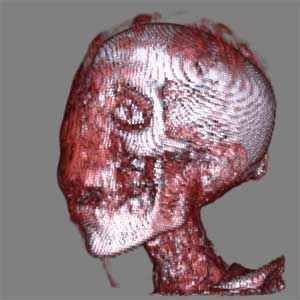Nearest Neighbor Interpolation

Trilinear interpolation is a process of location a point in three dimensions by linear interpolating in each dimension. Nearest neighbor merely sets a point value to the nearest actual value, and consequentially produces aliasing. As seen in the image above, this aliasing is clearly visible. Similarly to increasing the sample distance, the quality of nearest neighbor interpolation decreases as the eye moves closer to the image dataset. Each aliased voxel is magnified, which produces a mosaiced, blurry image, compared to the much smoother trilinear image.

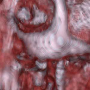Trilinear Interpolation, detail

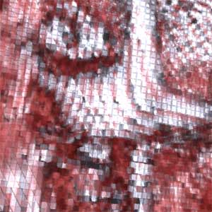Nearest Neighbor Interpolation, detail

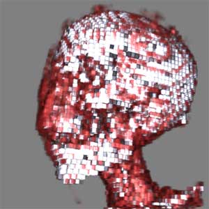
There are three provided dataset resolutions available. Naturally image quality is improved as the resolution increases, as illustrated below.

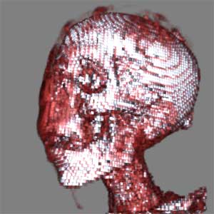
Resolution = 50	Resolution = 80
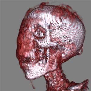
Resolution = 128

The higher resolution offers a much sharper, better defined image than at a resolution of 50. With each smaller resolution dataset, details are lost, which can reshape the image itself - the skull is rounder as well as softer at a resolution of 50. The skin in particular, which displays the extent of muscular preservation, becomes less defined at the lower resolution, as seen below. Other details vanish when shifting from a resolution of 80 to a resolution of 50, such as the bone structure of the eye, and the exact placement of the nose hole in the skull.

Resolution = 50

Resolution = 80

Finally, there is a relationship between the two interpolating methods (trilinear and nearest neighbor) at each resolution. Compared to the images above, which are rendered with trilinear interpolation, the below images suffer from the aliasing problems associated with nearest neighbor interpolation as well as the decreased resolution problems. The resolution decrease is plainly visible with nearest neighbor, as each voxel represents an increasingly large portion of the dataset. At a resolution of 50, each voxel is visible as a discrete, sharp block, compared to the trilinear images above, which interpolate across these blocks to produce a smoother, but blurrier image.

Resolution = 50	Resolution = 80
Resolution = 128