CS 6630 Scientific Visualization - Project 3
Zach Gildersleeve
Sept. 26, 2006
CADE login: gildersl
Graduate level credit
Part 1 - Contour Isosurfaces and Transfer Functions
Scripts Used: "contour.tcl"
Files Produced: images
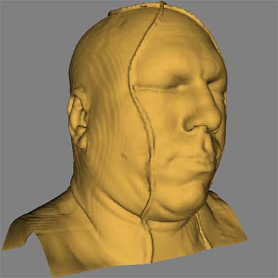
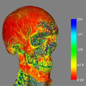
Isosurface contour value of 35
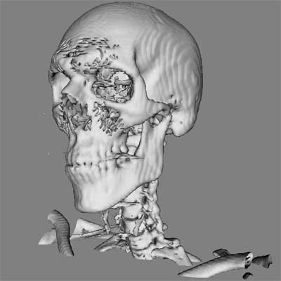
Isosurface contour value of 75
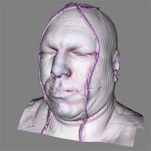
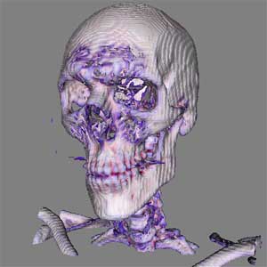
For the Visible Man head dataset, there are two isosurfaces ranges that provide useful information: the skin, and the bone. The skin isosurface lies in a range between 25 - 40, with the minimum amount of noise around a contour value of 35. The bone data in this scan is more varied than the skin, in that it lies in a much wider range. Contour values between 65 and 100 will return results, although the sinus region of the skull exists only very tentatively through the range of 65-80, but a value of 75 will provide clean results. The teeth portions of this dataset are exceedingly dense, and parts are still visible at a contour value of over 200, with a contour value of around 130 providing an interesting, if somewhat noisy and chunky, visualization of that region. Identifying these regions is a process of manually changing the contour value of the isosurface returned. This functionality is provided in the GUI in the form of a slider bar.
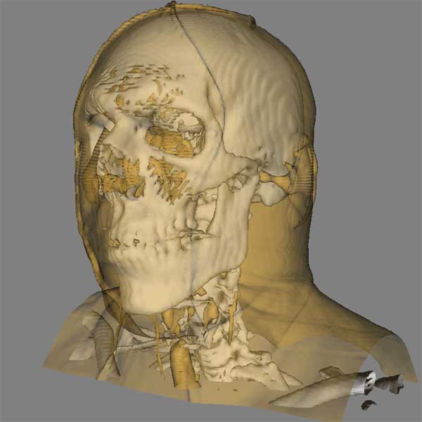
Using the above ideal contour values for the skin and bone, it is possible to combine the two isosurfaces using the transfer function approach to visualization of volume data. Assigning an opacity of 0.5 to the skin, and adding the two separate isosurfaces to the renderer produces the image below. One of the most interesting features of this visualization is the ear canal, as it is an area of skin / bone interaction that is not lost in the Visible Man's corpulence.
The GUI for "contour.tcl" provides four radio buttons. The user can select between the skin isosurface, the bone isosurface, the skin-bone transfer function, and an option to set the contour value manually, which opens a slider that controls the relative contour value. The pipeline is described below, and is duplicated for both the skin and bone isosurfaces.
structured points dataset -> structured points reader -> vtkContourFilter + set contour value -> vtkPolyDataNormals -> vtkPolyDataMapper (ScalarVisibilityOff allows for custom color) -> vtkActor + set color and opacity -> vtkRenderer
Univariate Color Mapped Volume
Script Used: "unicolor.tcl"
Files Produced: images
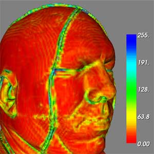 Skin isosurface with "norm" curvature |
 Bone isosurface with "norm" curvature |
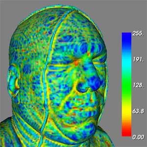 Skin isosurface with angle curvature |
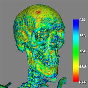 Bone isosurface with angle curvature |
When run, the script "unicolor.tcl" colors the above Visible Man head dataset with a univariate colormap, created in HSV colorspace. This colormap is applied to the generated isosurface using the contour values established above, and combined using vtkProbeFilter. The vtkProbeFilter computes point attributes at point positions, using the isosurface as the Input, and the colormapped dataset (via vtkImageMapToColors) as the Source. The rendering pipeline is very similar to the script detailed above:
structured points dataset -> structured points reader -> vtkImageMapToColors + built LUT
structured points dataset -> structured points reader -> vtkContourFilter + set contour value -> vtkPolyDataNormals
vtkProbeFilter + (Input = vtkPolyDataNormals) + (Source = vtkImageMapToColors) -> vtkPolyDataMapper -> vtkActor-> vtkRenderer
A GUI allows the user to switch between the skin and bone isosurfaces, and to separately switch between the different curvature values. Given the principle curvatures of the isosurface, k1 and k2, the "norm" values represent the total magnitude of the curvature (D = sqrt( k1 * k1 + k2 * k2). The trace angle value represents (k1 + k2) / D. The different between these two values is discussed below.
 Color mapped to "norm" curvature |
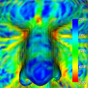 Color mapped to angle curvature |
The "norm" curvature represents the total magnitude of the curvature, that is, the greatest change in curvature from point to point. Examining the model, these points are found on the ears, alignment cords, nostrils, and the natural creases in the body. Overall, there is a smaller rate of change across the majority of the skin isosurface (shown in red above left), with understandably more variation in change of curvature magnitude on the bone isosurface, particularly on the neck vertebrae.
The trace angle curvature values represents what kind of curvature each point has, on a scale with very convex to very concave, and areas of relatively flat curvature in the middle (shown in green, above right). Thus, the tip of the nose on the skin isosurface and the tips of the teeth and chin in the bone isosurface are very convex surfaces, visualized in a full blue. The side of the nose between the eyes are highly concave surfaces, and are shown in red. This colormap reveals some interesting dimples on the skull, as seen on the bone isosurface, as well as mounds at the top and rear of the skull. However, the stairstepping of the dataset radiating from these points makes it difficult to understand what these different types of curvature correspond to in skeletal anatomy.
Angle curvature showing interesting variation (note saturated red and blue)
There is much more color variation in both the skin and bone isosurface with the angle curvature than the total magnitude curvature, and this corresponds to the generated isosurface itself. For example, the large patches of red using the "norm" curvature (low magnitude of curvature) correspond to an isosurface that is flatter from point to point. This seems fairly obvious after looking at the isosurfaces themselves. The colormap using the "norm" curvature does emphasize points that might be considered on an edge, which is useful, but nothing dramatic to the visualization of the isosurface. The trace angle curvature, on the other hand, reveals new elements about the underlying data, such as the dimples on the skull, the variation of the skin, and the tips of the vertebrae. In the end, the best visualization method is the one that best suits the particular need, but the degree to which the angle method isolates what could be considered key features is enlightening. The bivariate method described in the next section attempts to utilize the relevant portions of both curvature volumes at once, as we shall see.
Bivariate Color Mapped Volume
Script Used: "biColor.tcl"
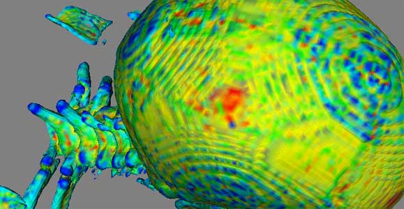
 Skin isosurface with anglenorm curvature data |
 Bone isosurface with anglenorm curvature data |
 The bivariate colormap employed |
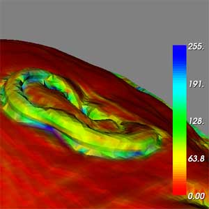
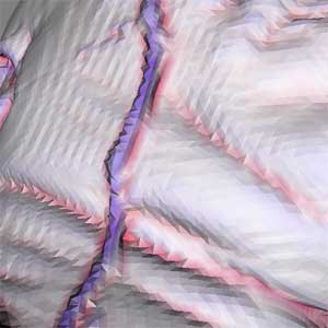 Detail of skin isosurface showing curvature |
The same skin and bone contour values were mapped with a multivariate colormap, using a similar workflow as above, with the inclusion of an anglenorm dataset that combines the norm and angle curvature into a multivariate volume, such that a bicolor look up table can be built and applied (see assignment 2 for the details of how to implement a bivariate colormap in VTK). In the colormap generated, the norm curvature (total magnitude of the curvature) varies horizontally from white to saturated color, and the angle (convex, concave, etc.) varies vertically from blue to red. As one might expect, the large patch of white in the colormap corresponds to where the norm is zero or very small. At these values, the colormap reflects that there is no corresponding angle to the curvature. Only when the norm gets sufficiently large does the angle of the curve become important, as seen on the right side of the colormap. When applied to the Visible Man head dataset, we see that most of the isosurface is white, meaning that most of the surface is relatively flat (and the angle of the curvature is meaningless.) This corresponds to the unicolor.tcl produced images with the norm curvature, with large portions of red signifying low curvature magnitude, but produces a much cleaner visualization. At the higher magnitude curvature, seen as green on the alignment cords in the same top univariate image, for example, the multivariate colormap displays the angle of the curvature, blue for highly convex, and red for highly concave. Thus, the bivariate colormap for this dataset combines the useful features from the norm and angle curvature volumes in one visualization, a significant accomplishment. The result is a clean visualization that illustrates multiple, relevant aspects to the data set.