CS 6630 Scientific Visualization - Project 1
Zach Gildersleeve
Sept. 26, 2006
CADE login: gildersl
Graduate level credit
Part 1 - Height Field Data
Thorax Data
Scripts Used: "writepoints.tcl", "viewThorax.tcl"
Files Produced: "thoraxPoints.vtk", images
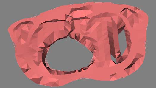
To visualize the thorax data requires first processing the condensing the assignment1.data and assignment1.pts into an appropriate format. This is done by writepoints.tcl, and produces a vtkPolyData stored in thoraxPoints.vtk. This dataset is run through a vtkDelaunay2D filter to tessellate the poly data into a viewable image, using a tolerance of 0.001 and an alpha of 18.0. When viewThorax.tcl is run, the user is presented with a visualization of the electric field potential of the selected 2D slice of the human thorax. The overall pipeline is as thus:
assignment1.pts + assignment1.data -> writepoints.tcl -> write - vtkPolyData - read -> vtkDelaunay2D filter -> vtk mapper -> vtk actor -> vtk renderer
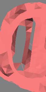
alpha = 15.0
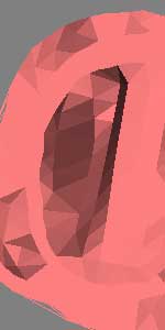
alpha = 20.0
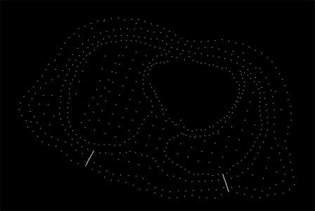
tolerance = 0.1, alpha is unused
This visualization raises several issues, which are illustrated in the above images. The delaunay tessellation is controlled via its tolerance and alpha settings. Too high an alpha level ( > 20.0 ) fills in the "holes" and creates solid surfaces where there are none. Too low an alpha value ( < 15.0 ) produces poor tessellation and artificial holes. This alpha range is unique to this dataset, and would almost certainly be different with other data. An accurate estimation of the most appropriate alpha range can be found by first raising the tolerance to a high value (0.1 with this data). This visualizes the discrete data points. Using a gestalt viewing mind set, the viewer can discern the natural shape of the data by viewing and rotating the data in 3D. Then, after lowering the tolerance (0.001) the viewer can manipulate the alpha range to best visually match the gestalt image. Further refinement of this process with interpolation, especially around the "holes" would produce in a physically accurate visualization.
Mount Hood Elevation Dataset
Script Used: "mtHoodWarp.tcl"
Files Produced: images
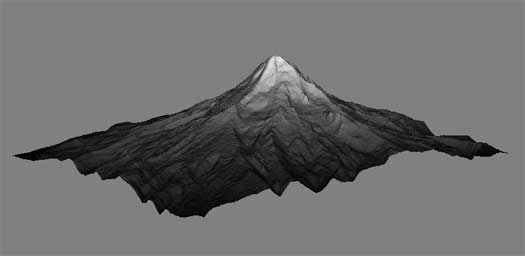
When run, the script mtHoodWarp.tcl allows the user to view a 3D representation of Mt. Hood. Interactivity is provided by vtkRenderWindowInteractor. The image is read in with vtkPNMReader, and the scalar grayscale values are used by vtkImageDataGeometryFilter and vtkWarpScalar to deform the geometry output. A warp scale factor of 0.25 is used to give the visualization the appropriate amount of height. The geometry and scalar filters are merged, sent to a mapper and then out to an actor. The pipeline is as follows:
grayscale image data -> read - vtkPNMReader -> structured points dataset -> vtkImageMagnitude -> image data to geometry filter -> vtkWarpScalar + scale factor -> geometry + reader merge -> vtk mapper -> vtk actor -> vtk renderer
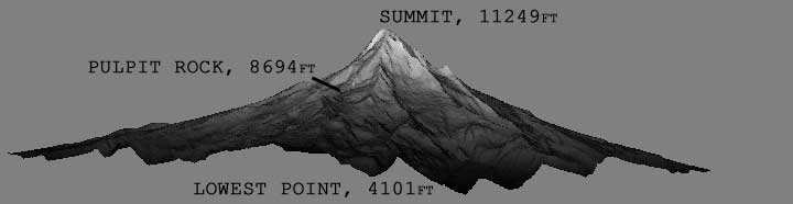
The appropriate warp scale factor was acquired by the following process. First, a rough idea of the Mt. Hood data scale was achieved by looking at topological maps of Mt. Hood. Two points in the dataset were selected to compute the scale, in this case the summit point, and Pulpit Rock, an outcropping north (dataset north) of the summit. By measuring the pixel distance between these two points in the dataset against the actual distance, an approximate scale of pixels per mile was acquired. Using a Photoshop selection filter, the lowest (blackest) pixel on the dataset was found, and the distance in pixel/miles from the summit to the lowest point was found. In a GPS mapping program, a circle with a radius of this distance was drawn from the summit, and the actual lowest elevation of the dataset was determined. From here a simple scaled ratio returned the scale of the dataset's lowest to highest point, in real world values, a ratio of very nearly 0.25.
Part 2 - Contour Maps
Script Used: "contour.tcl"
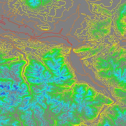
This script uses vtkContourFilter as the main filter for a series of structures point datasets. This filter produces isolines or isosurfaces based on the dataset, and the user must manually enter the contour values, based on a minimum and maximum contour level, as well as the number of intermediate contours. This is illustrated in the GUI, which allows the user to dynamically change these values. Different values produce dramatically different images, and the user must choose the appropriate settings, depending on the goal of the visualization. The script also provides a method to view the contours as a monotone image, or mapped through a rainbow color range. While the rainbow color variations are not tied to any specific contour value, the color helps to make sense of dense contour data, particularly with the brain MRI image, as illustrated in the images below.
The GUI provided by the contour.tcl script has three slider bars, all of which determine the look of the current image's contours. As described above, the user may adjust the number of contour lines, and the minimum and maximum value that the contour's represent. A set of radio buttons allows the user to select between the three datasets (body.vtk, brain.vtk, and topo.dem), and a second set of radio buttons allows the user to switch between a rainbow color scale and white. Note that the minimum and maximum contour value slider bars have values that range from -5000 to 5000, and default from 0 - 255 for the body and brain data. These values reflect that the source data is from a grayscale converted image, limited between those values, however interesting images can be created by moving the sliders beyond this value. The topo.dem sliders have different ranges based on the elevation range, and defaults to the lowest and highest elevation value for the data. The range of the number of contour lines is 0 - 50; an upper range for this slider above 50 tends to start filling in the image beyond the data present, resulting in a solid image and slower performance.
The GUI also includes a Camera Reset button, which will reset the rotation and zoom position of the camera relative to the active actor. It may be necessary to click in the window after pressing the Camera Reset button to force the window to update, especially when switching between the topo.dem data and the other two. This performance issue (on some systems contour.tcl was tested on) is most likely due to the large data size.
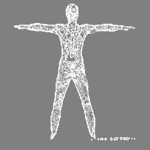
Body Data
This dataset is a grayscale conversion of an infrared scan of the human body, converted from full color. The pipeline for this visualization is as follows:
grayscale image data -> read - vtkStructuredPointsReader -> vtkContourFilter + generate contour values -> vtk mapper + scalar range -> vtk actor -> vtk renderer + GUI
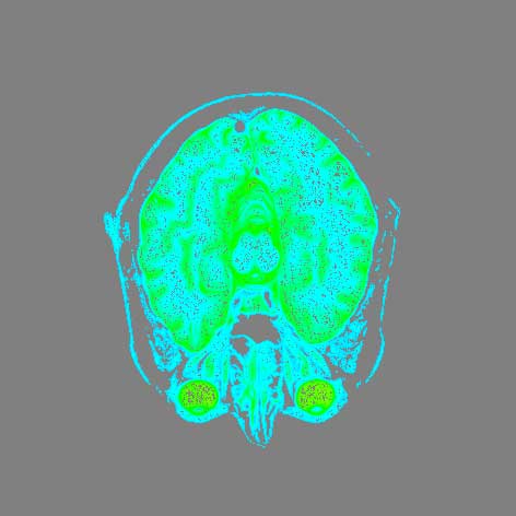
Brain Data
This dataset is a grayscale conversion of a DICOM (MRI) scan of the human brain. As is the body data, it is formatted in a format readable by vtkStructuredPointsReader, and follows the same workflow as the body data. The below image shows the brain data with the color map.
DEM Data
I got such a kick out of working with the Mt. Hood data above, and using mapping and topo tools to determine the accurate elevation scale, that I choose to work with DEM (Digital Elevation Model) data for the third image. DEM files depict elevation and topography by coordinates and elevation data, and do so in a raster format, compared with other elevation file formats that store topography as vectors. DEM files are the preferred base format for GIS (Geographic Information Systems), and are showing up in terrain rendering for simulations and film and media applications, which is where I have worked with the data before.
DEM files can be read by VTK using vtkDEMReader, however this returns a vtkImageData that contains scalar elevation data. This must be further processed to fit into the established vtkContourFilter pipeline. To surmount this hurdle, the DEM file is written to a file using vtkStructuredPointsWriter and then read into the pipeline from a file. Saving the file to disk results in better performance than converting the DEM file and writing and reading the structured points wholly in-script. This step could be necessary to re-write the DEM FORTRAN scientific notation exponent character with one used by C/C++. The DEM format has been superseded by the SDTS format, which is not yet directly supported by VTK. Due to the size of the DEM file, it may take a moment to respond to the GUI.
The workflow to process DEM files in the contour.tcl script is as follows:
DEM file -> read vtkDEMReader + get elevation bounds -> write vtkStructuredPointsWriter -> read - vtkStructuredPointsReader -> vtkContourFilter + generate contour values using elevation bounds -> vtk mapper + scalar range -> vtk actor -> vtk renderer + GUI
The following images show the DEM contour visualization, with different contour values. The DEM file shows part of Bozeman, Montana.
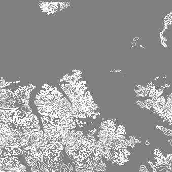
min = 2000, max = 3500, lines = 25
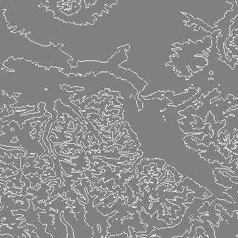
min = 1500, max = 3500, lines = 5
This data is interesting on several levels. First, topological data is very useful both for more traditional cartographic applications and for more creative applications like using DEM data for a realistic source for terrain rendering, particularly when matching the real world in visual effects for films. One method that I have worked through involved projecting photographic panoramas, taken from known geological points, onto DEM based geometry. The result is very realistic. The data is also interesting from an aesthetical point of view, as well as a demonstration of real-world fractals. It would be possible to isolate the fractal dimension of a DEM based terrain contour image, and then incorporate that dimension of fractal in terrain generation. Such a fractal dimension would vary from geographic location to location (i.e. Kansas vs. southern Utah), and an automatic fractal dimension acquisition tool via contouring could provide a hint of locality in terrain rendering.
Additional Questions
In order for a dataset to produce contour lines that make sense and contribute to visualization, the data must have some resemblance of order to it. That is, viewing a contour visualization of a very noisy sample will not be meaningful, likewise a very monotonous image. As mentioned in class, in 2D applications, contouring represents rate of change, and if this rate is near 0 or near 1, the visualization will be unenlightening. Of course, in these cases, one solution would be to shrink or enlarge the viewable area, but this may not be possible for all datasets. Essentially, there must be something to contour. Additionally, the dataset must be ordered in such a way as to allow for the contour to show relationships across the image. An dataset that has a exponent or logarithmic ordering to its samples will be contourable, but the contour lines will represent scalar values, and will be skewed to the high end. This, again is easy to correct, if known, but regular, discrete sampling helps produce cleaner contours.
Obviously, there are many examples of datasets that exhibit the above properties, and are well suited for contouring. Terrain and medial data, as those datasets seen above, can produce regular and discrete samples, and to do not have radical changes in slope. Any data that is capable of being viewed on a 2D plane, like weather patterns or environmental data such as population density or household income, fits these properties. Likewise, physical simulations of temperature or sound can be discretely sampled and then contoured.