CS 6620 Advanced Computer Graphics II - Assignment 8

Zach Gildersleeve
March 28, 2007

Required Image

Here are the required image, as produced by the program.

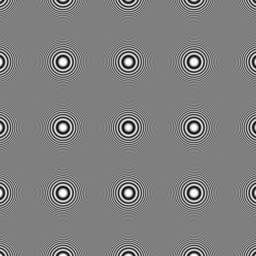
Above is the function 0.5 * (cos(500 * M_PI * (x * x + y * y)) + 1.0), rendered with one sample per pixel and no filtering. This is the same result as one sample per pixel and a box filter, using a support parameter of 1. Note that the center circle is the "true" function, and all other low frequency elements are alias's of the function's high frequency components.

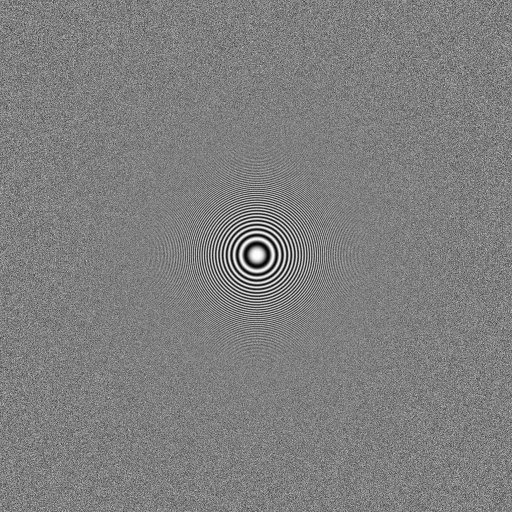
Above is the function filtered using a triangle with a support parameter of 2, and using 9 jittered samples per pixel. This filtered image starts to converge on the "true" function, at the expense of introduced noise.

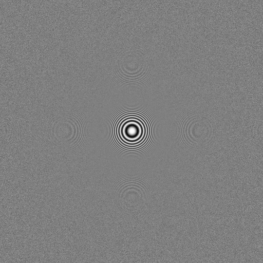
Above is the required function, filtered with a gaussian function with support parameter of 3, and using 9 jittered samples per pixel.

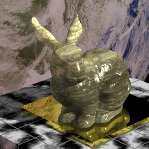
Here are the same set of filters, applied to an image.

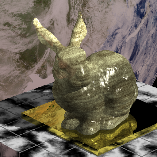
Above is the image rendered with one uniform sample per pixel and a box filter with support parameter of 1. This image took 109 seconds to render.

Above is the image rendered with 9 jittered samples per pixel, using a triangle filter with support parameter of 2. This image took 2409 seconds to render, or 40.15 minutes.

Above is the image rendered with 9 jittered samples per pixel, using a gaussian filter with support parameter of 3. This image took 3552 seconds to render, or 59.2 minutes. As might be expected, the gaussian looks slightly more blurred than the triangle filter.

Code Listing

The code for this image can be found here.

All images produced for this assignment can be found here.

Design Choices

This project is centered around two new classes, Filter and Sampler. Sampler describes two types of sampling methods, Uniform and Jittered. All pixels that are multisampled are represented as arrays. When passed to the Sampler, these arrays, given the x and y value of the pixel and the pixel neighborhood support required, are loaded with either the center subpixel coordinate value or a random set of subpixel coordinate values, expressed in subpixel coordinate space. Filter similarly has several child classes - BoxFilter, TriangleFilter, GaussianFilter - that are passed in the same pixel array, as well as an array of weights. Each element in the array of weights represents the weighted value of the subpixel sample at that respective index in the sampled coordinate array set. Using different functions returns different weights per sample.

The rendering function in Scene also has some changes to incorporate the Sampler and Filter classes into each Scene. This is also expressed in the class ImageProcessing, which combines elements from main.cpp, prog0*.h, and Scene to render the cosine function for the required images above. For each pixel in the rendering double loop, the weight and 2D subpixel coordinate arrays are initialized given the square of the number of samples. The above mentioned methods to get the sample subpixel coordinates as well as the weights is called. The samples are looped over, with the object intersection routine being called for each sample. The resulting ray color is multiplied by the previously computed weight of that respective sample, and all the resulting sampled colors are summed, then divided by the total weight to return the filtered value of the pixel. No reuse of pixels was implemented, thus for the required images rendering took much longer than without filtering or sampling.

Extra Credit

The bunny scene was rendered at 1024 x 1024 and then transformed to the frequency domain for the below images. This was done in MatLab. The image was converted to grayscale, then transformed, shifted, and scaled appropriately. The pseudocode to accomplish this is:

convert to grayscale;
read in image as doubles;
ft = fftshift(fft2(image);
ft = log(abs(ft) + 1);
find min and max of ft
ft = (ft - min) / (max - min);
display image

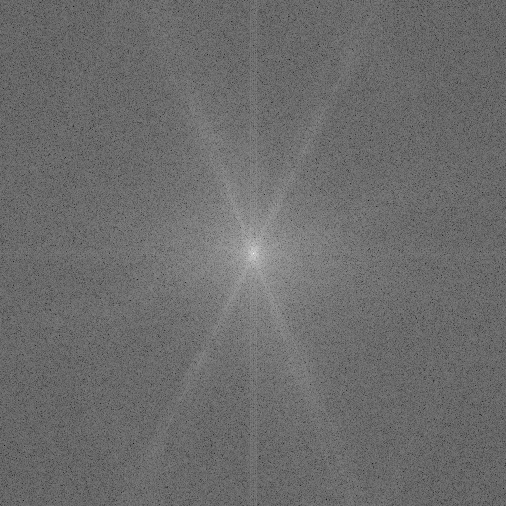
The above image is a visualization of the frequency spectrum of the bunny scene, rendered with 1 uniform sample per pixel and filtered using a box filter with a support parameter of 1. This scene at 1024 x 1024 took 221 seconds to render, or 3.68 minutes.

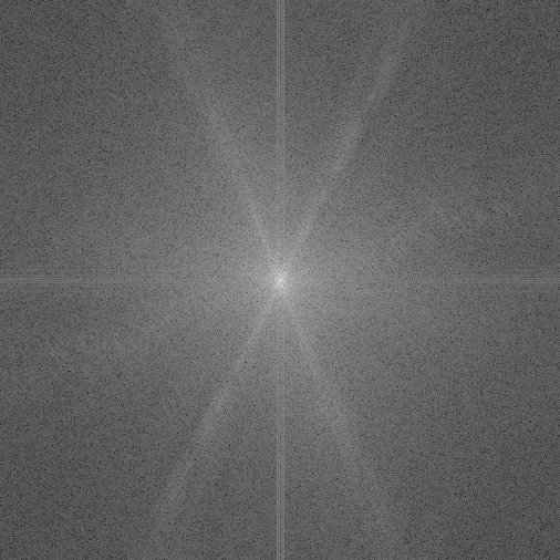
The above image is a visualization of the frequency spectrum of the bunny scene, rendered with 9 jittered samples per pixel and filtered using a triangle filter with a support parameter of 2. This scene at 1024 x 1024 took 5248 seconds to render, or 87.46 minutes. Note the increased definition of the power bands, and the broad band now visible running from approximately 60 degrees CW from top center (2 o'clock) to 240 degrees CW (8 o'clock).

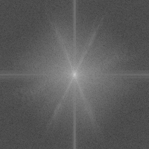
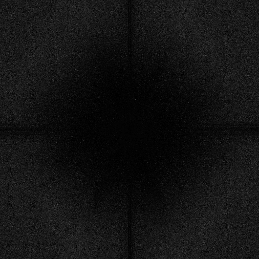
The above image is a visualization of the frequency spectrum of the bunny scene, rendered with 9 jittered samples per pixel and filtered using a gaussian filter with a support parameter of 3. This scene at 1024 x 1024 took 10035 seconds to render, or 2.79 hours.

Finally, here is the difference between the gaussian frequency spectrum and the box filter frequency spectrum, which demonstrates the removal of high frequency elements by the gaussian filter, while still maintaining the lower frequencies.

Additional Comments

The first set of required images (sinc function) took me about 8 hours, and included the Sampler and Filter classes, which are fairly straightforward. I had several bugs while linking the Filter and Sampler into the Scene pipeline, which took another 6 or so hours to troubleshoot. In my Scene::render() function I was not properly initializing a new HitRecord for every sub-sample, which made only the left edges of a Primitive filter correctly, and produced errors in the reflection. I spent under an hour producing the frequency domain images for the extra credit. The times specified here do not include rendering. The images shown in this report represent around 6 hours of rendering time; total rendering time spent on this assignment was well over 20 hours.